


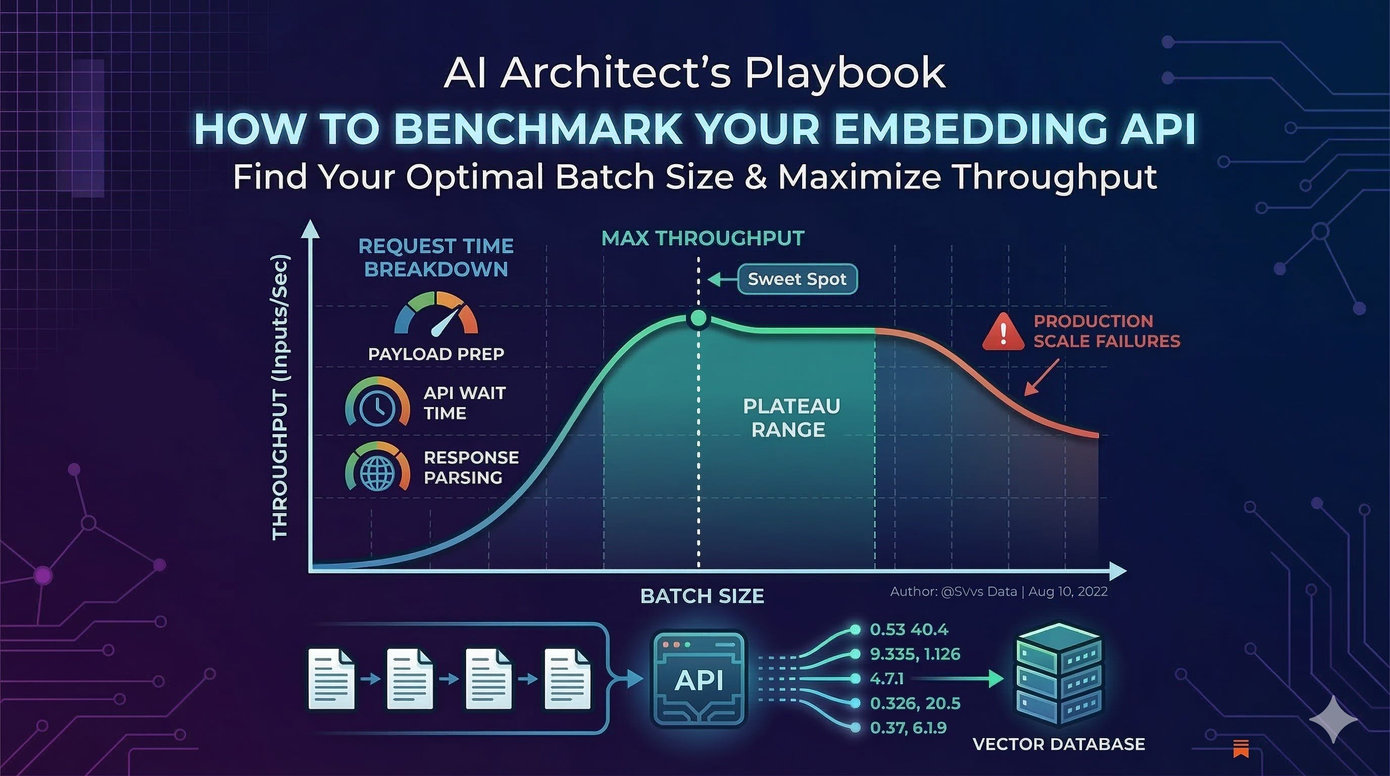
When you build an application that uses embedding models - whether for semantic search, retrieval-augmented generation, or any other vector-based workflow - measuring performance is easy to put off. You get the feature working, the embeddings look right, and you move on.
Then someone asks: “How long will it take to vectorize our 50 million documents?”
If you have not done the performance work by that point, the question becomes a problem without a quick answer. I have been there. This post is about doing that work before you need the answer, building a repeatable performance testing approach rather than figuring it out under pressure.
One clarification on scope: this guide focuses specifically on batch embedding generation - sending multiple text inputs to an embedding API in a single call and measuring the throughput. If you are calling an embedding API one input at a time, some of this still applies, but the biggest gains described here come from batching. That context matters as you read.
I will walk through the performance testing approach I have been developing and refining through real experiments against cloud embedding APIs and a self-hosted vLLM endpoint. The work ranged from small single-request tests all the way to running embedding generation over datasets at million-row scale.
Why Embedding APIs Warrant Their Own Performance Testing Approach
Embedding APIs are used differently from text generation APIs, and that difference shapes how you should think about performance.
With a generation API, you typically process one request at a time - a user sends a prompt, the model responds. With an embedding API, you are almost always working in bulk. A product catalog with 10 million descriptions needs all 10 million vectorized. A document corpus gets re-indexed every night. The volume is large, and it often runs as a background job where throughput matters more than single-request response time.
This bulk processing nature means that small configuration choices - like batch size - can have large effects on the total time and cost to complete a job. For example, running with a poorly chosen batch size can cut your throughput significantly compared to an optimized one, and that difference compounds across every run, every day, at every scale. It is not the only thing that matters, but it is one of the most controllable levers you have.
The performance testing approach covered here focuses on four questions:
What limits does your embedding API put on each call?
At what batch size does throughput peak for your model and data?
How does throughput drop when you go past that batch size?
What breaks when you run the same job at production scale?
Step 1: Know Your API’s Hard Limits Before You Test Anything
Before running a single test, check the documentation for your embedding provider and answer one question: how does this API limit what you can send in a single call?
There are two common patterns:
Input count limits. Some providers cap the number of text inputs you can include in one API call. Once you exceed that number, the request is rejected. Always verify the current limit in the provider’s documentation, as these can change.
Token budget limits. Other providers do not set an input count limit directly, but cap the total number of tokens across all inputs in a single call. For example, if the limit is 300,000 tokens and your texts average 450 tokens each, that budget translates to roughly 666 inputs per call. The limit is not stated as an input count, but it effectively becomes one based on your data.
These two approaches require different batching logic. With an input count limit, you can set a fixed maximum batch size. With a token budget, your effective batch size depends on the actual token length of your inputs, so you need to calculate it dynamically for each batch rather than hardcoding a number. Getting this wrong - for example, assuming all inputs are short when some are long - can cause unexpected failures partway through a large job.
All of the APIs I tested were REST APIs. The limits below reflect what the REST API accepts per call. These figures come from publicly available documentation at the time of writing. Always check the provider's current docs before using them, as limits can change.
WatsonX AI — Input count limit. Observed up to 1,000 inputs per call in my own testing. IBM Cloud API Docs
OpenAI — Token budget. 300,000 tokens total across all inputs per call. OpenAI API Reference
Azure OpenAI — Input count limit. Up to 2,048 inputs per array per call. Azure OpenAI docs
AWS Bedrock (Titan) — Single input only. The InvokeModel REST API accepts one input string per call — batch arrays are not supported. AWS docs
vLLM (self-hosted) — Depends on deployment. The server operator controls limits at startup via
--max-num-batched-tokensand--max-num-seqs. In my own testing I was able to send up to 10,000 inputs in a single call. vLLM Engine Arguments
A note on counting tokens before you send them. If your provider uses a token budget, you need a way to estimate token counts on your side before constructing each batch. Calling the API itself to count tokens is expensive and defeats the purpose. A practical alternative is to use an open-source tokenizer locally. For OpenAI-compatible APIs, the tiktoken Python library can count tokens offline at no API cost. For other models, the transformers library from Hugging Face provides tokenizers that run locally. Neither requires a network call, and both run quickly enough to be part of your batching logic at scale.
Step 2: Measure the Right Things - Break Down Where Time Goes
Before you start adjusting batch sizes, set up your measurement code to separate request time into three distinct parts. This is easy to skip, but it is where the most useful diagnostic information comes from.
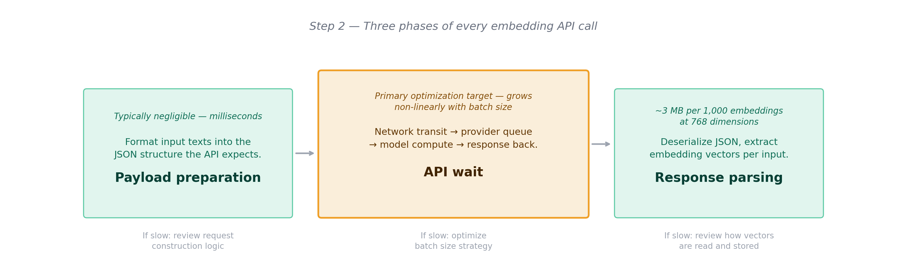
Payload preparation is the time your code spends building the request - formatting your list of input texts into the JSON structure the API expects. For small batches, this is negligible. For large batches with many long texts, it can add up and become worth optimizing separately.
API wait is the time from when your request leaves your machine to when the response starts coming back. This includes network travel time in both directions, any time the request spends waiting in a queue on the provider’s side, and the time the model actually takes to compute the embeddings. This phase typically takes the most time, and it grows with batch size - though not in a straight line, as you will see in Step 3.
Response parsing is the time your code spends reading the response and extracting the embedding vectors. At larger batch sizes, responses get large. A batch of 1,000 embeddings at 768 dimensions, stored as 32-bit floats, contains about 3 MB of numerical data to read and process. Measuring this separately helps confirm whether response handling is ever a bottleneck.
When you break latency into these three parts, you can see where to focus. If API wait is the dominant cost, then batching strategy is your main lever. If payload prep is surprisingly slow, look at how you are constructing requests. If response parsing takes longer than expected, look at how you are reading and storing results.
Step 3: Find Where Throughput Peaks - and Where It Falls Off
This is the core of the performance testing work. The goal is to find the batch size where you get the most inputs processed per second, and to understand what happens on both sides of that point.
When you plot throughput against batch size, you get a curve with a predictable shape: it rises quickly at first, peaks somewhere in the middle, and then gradually declines. Three things drive that shape:
Why throughput rises as batch size increases. Every API call has a fixed cost you pay regardless of how many inputs are in it: the time to establish the connection, send the request, and receive the response. At batch size 1, that fixed cost is most of your total call time. At batch size 10, you pay the same fixed cost but process 10 inputs instead of 1, so your throughput is roughly 10 times higher. As batch size grows, that fixed cost gets spread across more inputs and throughput climbs.
Why throughput eventually stops climbing. Once the batch is large enough, the fixed overhead is fully spread out and the model’s compute time per input becomes the main cost. Throughput levels off. This is the plateau.
Why throughput can drop with very large batches. Very large batches introduce new costs: larger payloads take longer to send over the network, the server may need to split your batch into smaller internal chunks to process it, and memory pressure on the server side increases response time. The result is that throughput can actually decrease beyond a certain point, even though more data is being sent.
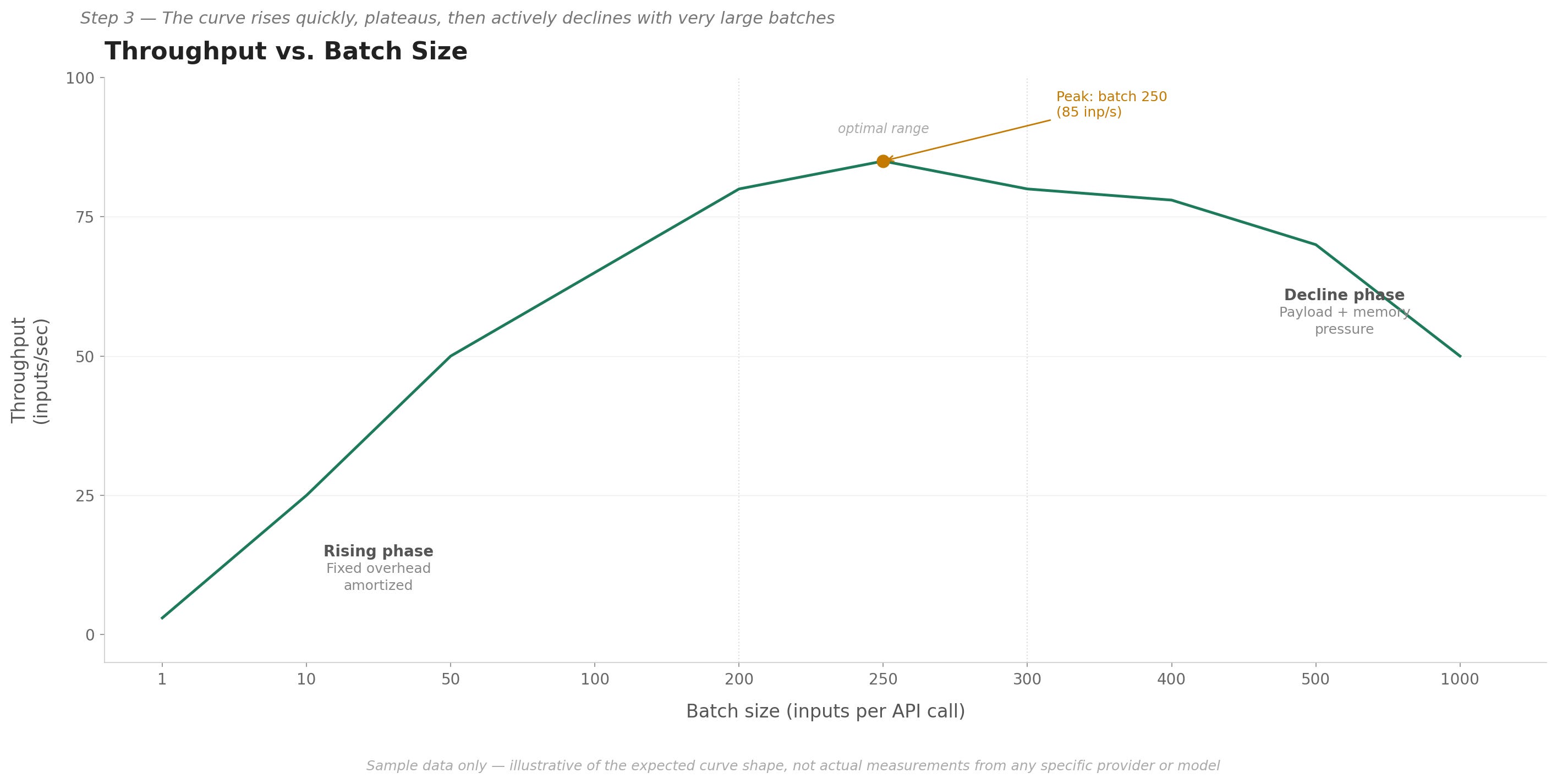
A few patterns worth noting in this kind of result:
Batch sizes 1 and 10 can have nearly the same total call time (both around 0.4 seconds in this example), yet batch 10 delivers about 10 times the throughput. This is the fixed-cost effect at its clearest - you are doing 10 times the work for no additional waiting time.
The provider’s maximum allowed batch size is often not the most efficient one. In this sample, batch 1,000 - the largest - produces the lowest throughput. The API accepting a batch size does not mean that size is the best choice.
The peak is typically a range, not a single number. In the sample above, batch sizes from about 200 to 300 all deliver throughput within 5-10% of the peak. This is useful in practice: if your batches are not always exactly the same size, anything in that range will perform similarly well.
How to run this test. Pick a fixed dataset of text inputs with a consistent average length (matching your real workload as closely as possible). Start with batch size 1 and work up through increasing sizes - for example, 1, 10, 50, 100, 200, 250, 300, 400, 500, up to your provider’s maximum. For each batch size, run at least three separate calls and average the results to reduce the effect of network variation. Include one unmeasured warm-up call at the start of each batch size to avoid counting any startup effects in your measurements.
Step 4: Test Each Model Separately
The batch size that gives the best throughput is not the same for every model. Smaller models compute embeddings faster per input, so they can handle larger batches before hitting the plateau. Larger models take more compute time per input, so the plateau arrives at a lower batch size, and the performance drop from oversized batches tends to be steeper.
When I ran the same batch size test across three models of different sizes - small (around 30M parameters), medium (around 125M), and large (around 500M or more) - the curve shape was similar for all three, but the peak location and the absolute throughput values were different for each. Larger models peaked at a lower batch size and at lower throughput overall.
The takeaway is simple: if you are working with more than one embedding model, run the batch size test for each one independently. Do not carry over the optimal batch size from a small model and assume it applies to a larger one.
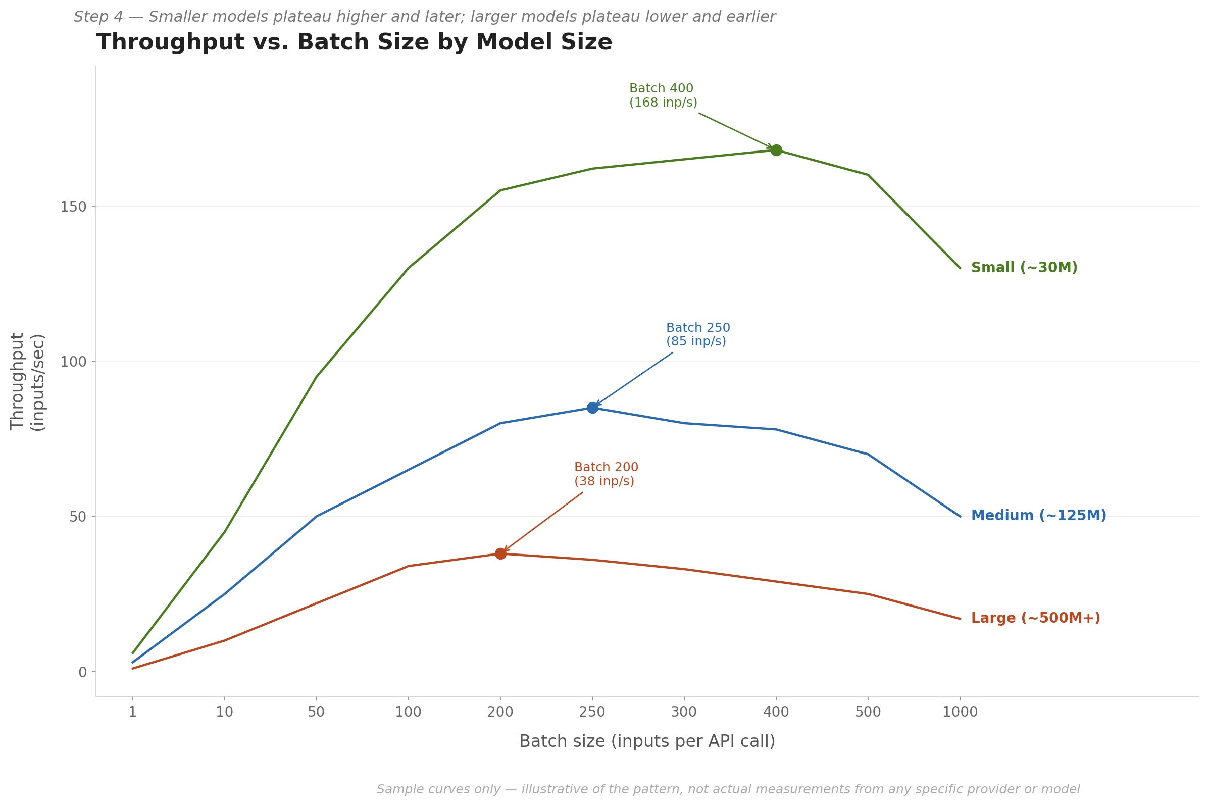
To keep the comparison clean, hold everything else constant - the same input texts, the same infrastructure, the same measurement approach. Change only the model. This way, any difference in results can be attributed to the model rather than noise from other variables.
Step 5: Test With Different Input Lengths
Most performance tests use a fixed text length, but real data rarely has perfectly uniform length. The token length of your inputs affects throughput in ways that are worth understanding before you run your tests, and it affects providers differently depending on whether they use input count limits or token budget limits.
A practical way to test this is to prepare separate datasets at a few different average token lengths - for example, a short-text set (around 50 tokens per input, like product titles or search queries), a medium-text set (around 150 to 250 tokens, like short paragraphs), and a long-text set (around 400 to 500 tokens, like full document sections). Run the same batch size test on each.
With short texts, you can fit more inputs within a token budget per call, but the fixed API overhead becomes a larger proportion of your total time per input. With long texts, your effective batch size shrinks if you are working within a token budget. The optimal batch size by input count may be quite different across these three workloads.
One specific edge case worth testing: what happens when an input exceeds the model’s maximum token length? Some APIs truncate the input silently and return an embedding anyway. Others return an error. Others may return something that looks like a valid embedding but reflects only part of the input. The behavior varies by provider and model, and it is worth verifying directly for your setup rather than assuming. If your real data has any inputs that might be unusually long, this test can prevent silent failures in production.
Step 6: Test at Real Scale
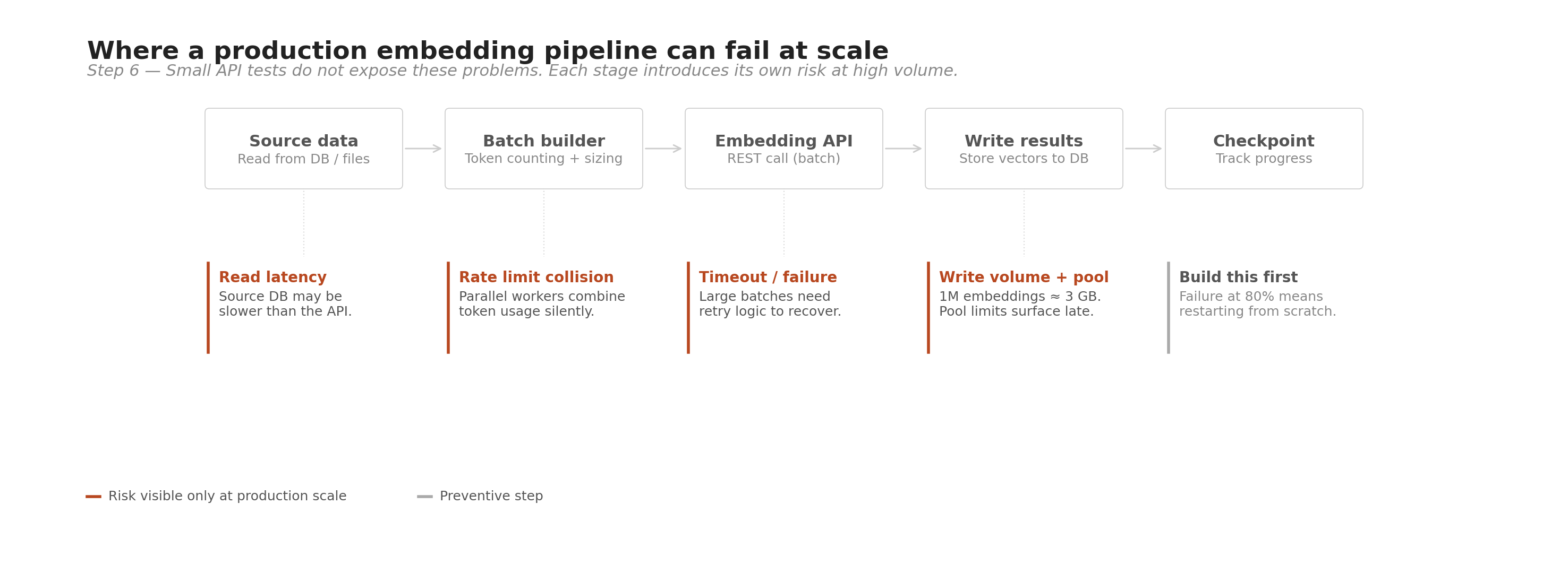
Small tests tell you how the API behaves call by call. They do not tell you what happens when you run a job across millions of inputs over several hours. Scale introduces a different set of problems, and many of them only become visible once you are running at that size.
I will not share specific numbers from my own large-scale experiments here, as that work was done in a professional context. But the problems I ran into are common enough to be worth sharing.
The bottleneck often is not the API. When running a long embedding job end to end, the slowest part is not always the embedding API call. Time spent reading inputs from the source system, writing results back to storage, and handling coordination between parallel workers can all add up. Measure the full pipeline, not just the API call times, to find where the real time goes.
Write volume adds up at scale. Embedding vectors are not small. At 768 dimensions stored as 32-bit floats, each embedding is exactly 3 KB. Writing 1 million embeddings means writing just under 3 GB of data. If you are writing to a database or storage system that has transaction or write limits, those limits can become a bottleneck or cause failures mid-job. Check the limits of your write destination before starting a large run, not after hitting an error.
Concurrent API calls and token rate limits interact. Running multiple parallel workers to call the embedding API at the same time can speed things up significantly. But if the provider has a rate limit measured in tokens per minute, the token usage from all your parallel workers adds up together. It is easy to hit a rate limit mid-job when running in parallel even if no single worker would hit it on its own. Test your parallel configuration against the provider’s rate limits before committing to it at full scale.
Connection pool limits surface late. If your parallel workers each hold a database connection for writing results, the total number of concurrent connections can exceed your connection pool limit. This type of failure often does not show up until you are partway through a large job. Test with enough scale to expose it before running the full job.
Build resume capability before you need it. A job processing a million inputs that fails at 80% completion should be able to pick up where it left off, not start over. This is straightforward to build before you start a large run and very difficult to add after you have already failed and need to rerun. Track which inputs have been successfully processed and skip them on restart.
Step 7: Run Multiple Iterations and Look at Consistency
A single measurement tells you what happened once. API performance varies based on server load on the provider’s side, network conditions between you and the provider, and the time of day the call is made. A result from one run may not reflect what you will see reliably in practice.
Running each batch size configuration at least three times and looking at the spread of results gives a more reliable picture. If the three results are close together, you can be more confident in the average. If one run is significantly different from the others, that variance is itself useful information - it tells you that the performance at that configuration is less predictable, which matters for planning.
In my own tests, mid-range batch sizes tended to show more variation between runs than very small or very large ones. The practical lesson: when planning how much headroom to build into a performance estimate for a production job, do not base it only on the best case from a small number of test runs. Look at the range of results and plan for something closer to the typical case, not the best one.
Putting It Together: A Testing Checklist
Here is a checklist that pulls together the steps above. Use it as a starting point and adjust it to your situation.
Before you start testing:
Find the current documented limits for your embedding API (input count or token budget).
Determine whether you need static batch sizes (input count limit) or dynamic batch sizing (token budget).
Set up local token counting so you can estimate batch sizes without API calls (e.g.,
tiktokenfor OpenAI-compatible APIs).Instrument your code to separately measure payload preparation time, API wait time, and response parsing time.
Prepare representative test datasets at short, medium, and long average token lengths.
Running the batch size test:
Test batch sizes from 1 up to the provider’s maximum, using regular intervals.
Run at least three iterations for each batch size.
Use one unmeasured warm-up call at the start of each batch size series.
Change only one variable at a time across test runs.
Repeat the test for each embedding model you plan to use.
Edge cases to verify:
What happens when an input exceeds the model’s maximum token length?
What happens when you approach or exceed the provider’s rate limit?
How does performance vary when input lengths within a single batch are uneven?
Scaling to production volume:
Test the full pipeline end to end, not just the API calls
Check write volume and storage limits for your target system at scale
Test parallel worker configuration against the provider’s rate limits
Verify connection pool limits under your expected concurrency level
Build and test checkpoint and resume functionality before running at full scale
Run at an intermediate scale (for example, 1% or 10% of your target volume) before committing to the full job
Closing Thought
The biggest performance gain in embedding batch workloads does not require new hardware, a faster model, or a different provider. It comes from batching correctly.
Two API calls that take the same time can have very different throughput — one sending a single input, the other sending a well-sized batch. The larger batch processes many more inputs for the same cost. At the scale embedding pipelines typically run, that difference translates directly into hours of processing time and real infrastructure cost.
The numbers will look different for every model, workload, and provider. The method for finding them does not change.
If you have run similar experiments or found different patterns, I would be curious to hear about it in the comments.
All experiments were run from my personal machine calling external APIs. Any numbers shown are illustrative samples only - they demonstrate the shape of results, not actual measurements from any specific provider. These are personal observations and do not represent my employer or any official benchmark.